22. Parametric Surfaces and Surface Integrals

c. Scalar Surface Integrals

1. Grid Cells and Scalar Surface Area Differential

We have learned how to integrate over curves and regions in \(\mathbb{R}^2\) and \(\mathbb{R}^3\). We want to learn how to integrate over surfaces in \(\mathbb{R}^3\). The process is always the same: chop up the surface into small pieces, calculate something on each piece and add them up. Integrating over a parametric surface in \(\mathbb{R}^3\): \[ (x,y,z)=\vec R(u,v)=\left\langle x(u,v),y(u,v),z(u,v)\right\rangle \] is most like integrating over a region in \(\mathbb{R}^2\) in curvilinear coordinates: \[ (x,y)=\vec R(u,v)=\left\langle x(u,v),y(u,v)\right\rangle \] In fact, a curvilinear coordinate system for a region in \(\mathbb{R}^2\) is actually just a parametric surface which happens to lie in the \(xy\)-plane, i.e. \(z=0\). Here again are the coordinate grids for a curvilinear coordinate system in \(\mathbb{R}^2\) and for parametric surface in \(\mathbb{R}^3\).

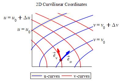
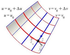
In both cases, the blue curves are \(u\)-curves because \(u\) is changing and are labeled by a value of \(v\).
Similarly, the red curves are \(v\)-curves because \(v\) is changing and are labeled by a value of \(u\).

In both cases, in order to integrate, you need to know (or be able to approximate) the area of a coordinate grid box: \[ u_0 \le u \le u_0+\Delta u \qquad \qquad v_0 \le v \le v_0+\Delta v \] For a curvilinear coordinate system, we call this area \(\Delta A\). For a parametric surface, we call this area \(\Delta S\) for surface area. The process of computing \(\Delta S\) is completely analogous to that for computing \(\Delta A\). We first compute the coordinate tangent vectors \[ \vec{e}_u=\dfrac{\partial\vec R}{\partial u} \qquad \text{and} \qquad \vec{e}_v=\dfrac{\partial\vec R}{\partial v} \] and add them to the plots:

PY: Rotate plot so e_u is visible. Actually move this down and put here a plot without the normal.

Next we stretch (or shrink) the coordinate tangent vectors, \(\vec{e}_u\) and \(\vec{e}_v\), into vectors, \(\vec{U}\) and \(\vec{V}\) resp., which just touch the next coordinate curve. (The magnitude is equal to the arc length of the coordinate curve.)

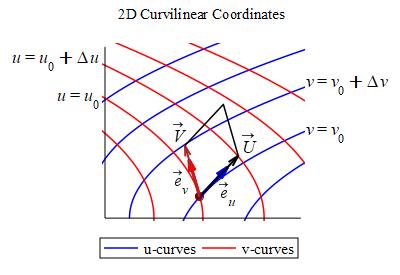
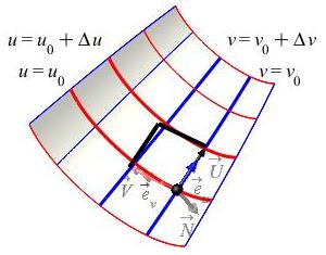
In both cases, we approximate the area of the coordinate grid box by the area of the parallelogram with edges \(\vec{U}\) and \(\vec{V}\) which is the magnitude of the cross product of \(\vec{U}\) and \(\vec{V}\). \[ \Delta A\approx|\vec{U}\times\vec{V}| \qquad \text{and} \qquad \Delta S\approx|\vec{U}\times\vec{V}| \] In both cases, we approximate \(\vec{U}\) and \(\vec{V}\) as: (See the derivation on this page.) \[ \vec{U}\approx\vec{e}_u\,\Delta u \qquad \text{and} \qquad \vec{V}\approx\vec{e}_v\,\Delta v \] So the areas become \[ \Delta A\approx|\vec{e}_u\times\vec{e}_v|\,\Delta u\,\Delta v \qquad \text{and} \qquad \Delta S\approx|\vec{e}_u\times\vec{e}_v|\,\Delta u\,\Delta v \] In the limit as \(\Delta u\) and \(\Delta v\) get small, these become the (scalar) differential of area, \(dA\), and the (scalar) differential of surface area, \(dS\). \[ dA=|\vec{e}_u\times\vec{e}_v|\,du\,dv \qquad \text{and}\qquad dS=|\vec{e}_u\times\vec{e}_v|\,du\,dv \] For the curvilinear coordinate system, we found that the length of the cross product of the tangent vectors was the Jacobian factor which is the absolute value of the Jacobian determinant: \[ |\vec{e}_u\times\vec{e}_v|=J =\left|\dfrac{\partial(x,y)}{\partial(u,v)}\right| =\left| \begin{vmatrix} \dfrac{\partial x}{\partial u}&\dfrac{\partial y}{\partial u} \\ \dfrac{\partial x}{\partial v}&\dfrac{\partial y}{\partial v} \end{vmatrix} \right| \] For the parametric surface, we recognize that the cross product of the tangent vectors is the normal vector: \[ \vec N=\vec{e}_u\times\vec{e}_v =\left\langle \dfrac{\partial(y,z)}{\partial(u,v)}, \dfrac{\partial(z,x)}{\partial(u,v)}, \dfrac{\partial(x,y)}{\partial(u,v)}\right\rangle \] So the length of the cross product is the length of the normal vector: \[ |\vec{e}_u\times\vec{e}_v|=|\vec{N}| =\sqrt{ \left(\dfrac{\partial(y,z)}{\partial(u,v)}\right)^2 +\left(\dfrac{\partial(z,x)}{\partial(u,v)}\right)^2 +\left(\dfrac{\partial(x,y)}{\partial(u,v)}\right)^2} \] So the differentials of area and surface area become \[ dA=J\,du\,dv \qquad \text{and} \qquad dS=|\vec{N}|\,du\,dv \]

Although the length of the normal, \(|\vec{N}|\), plays the roll of the Jacobian in the differential of surface area, it is technically NOT a Jacobian because it is not simply the determinant of the partial derivatives of \(2\) variables with respect to \(2\) variables.

In the above derivation, the scalar differential of surface area, \(dS\), was analogous to the differential of surface area, \(dA\). However, in computing integrals, the scalar differential of surface area, \(dS\), is actually more analogous to the scalar differential of arc length, \(ds\).

For a parametric curve, the important vector is the tangent vector, \(\vec{v}\).
For a parametric surface, the important vector is the normal vector, \(\vec{N}\).

We previously learned that the scalar differential of arc length is: \[ ds=|\vec{v}|\,dt \] We now have

The scalar differential of surface area is \[ dS=|\vec{N}|\,du\,dv \]

The lengths of the important vectors appear before the differentials. Notice the lower case \(s\) for curves and the upper case \(S\) for surfaces.

We previously learned that there is also a vector differential of arc length. In a few pages you will learn about the vector differential of surface area. These are \[ d\vec{s}=\vec{v}\,dt \qquad \text{and} \qquad d\vec{S}=\vec{N}\,du\,dv \] Now the important vectors themselves appear before the differentials. Notice the parallels.

We are finally ready to compute surface integrals.